Analysing results
End results
In the first tutorial you solved a very simple DCOP using the following command:
pydcop solve --algo dpop graph_coloring.yaml
This command outputs many results, given in json so that you can parse then
easily, for example when writing more complex scripts for
experimentation.
You can also get these results directly in a file using the --output global
option (see. pyDcop cli dcoumentation):
pydcop --output results.json solve --algo dpop graph_coloring.yaml
You may have noticed that, even though the DCOP has only 3 variables and a handful of constraints, the results file is quite long and contains a lot of information.
At the top level you can find global results, which apply to the DCOP as a whole:
{
  "agt_metrics": {
    // metrics for each agent, see below
  },
  "assignment": {
    "v1": "R",
    "v2": "G",
    "v3": "R"
  },
  "cost": -0.1,
  "cycle": 1,
  "msg_count": 29,
  "msg_size": 8,
  "status": "FINISHED",
  "time": 0.006329163996269926,
  "violation": 0
}
status: indicates how the command was stopped, can be one ofFINISHED, when all computation finished,TIMEOUT, when the command was interrupted because it reached timeout set with the--timeoutoption,STOPPED, when the command was interrupted withCTRL+C.
assignment: contains the assignment that was found by the DCOP algorithm.cost: the cost for this assignment (i.e. the sum of the cost of all constraints in the DCOP).violation: the number of violated hard constraints, when using DCOP with a mix of soft and hard constraints (hard constraint support is still experimental and not documented).msg_size: the total size of messages exchanged between agents.msg_count: the number of messages exchanged between agents.time: the elapsed time, in second.cycles, the number of cycles for DCOP computations. In this example it is always 0 has DPOP has no notion of cycle.
The agt_metrics section contains one entry for each of the agents in the
DCOP. Each of these entries contains several items:
"a1": {
  "activity_ratio": 0.24987247830102727,
  "count_ext_msg": {
    "v2": 2
  },
  "cycles": {
    "v2": 0
  },
  "size_ext_msg": {
    "v2": 4
  }
},
count_ext_msgandsize_ext_msg, which contain the count and size of messages sent and received by each DCOP computation hosted on this agentcycles, the number of cycles for each DCOP computation hosted on this agent. In this example it is always 0 because DPOP has no notion of cycle.activity_ratio, the ratio of active time to total elapsed time,where active time is defined as the time the agent spent handling a message as opposed to waiting for messages.
Run-time metrics
The output of the solve command only gives you
the end results of the command, but sometimes you need to know what happens
during the execution of the DCOP algorithm.
pyDCOP is able to collect metrics at different events during the DCOP execution.
You must use the --collect_on option to select
when you want metrics to be captured:
cycle_change: metrics are collected every time the algorithm switch from one cycle (aka iteration) to the next one. This mode only makes sense with algorithms which have a notion of cycle.period: metrics are collected periodically , for each agent (meaning your will have line of metric for each agent and for each period). When using this mode, you must also set--periodto set the metrics collection period (in second).value_change: metrics are collected every time a new value is selected for a variable.
When collecting run-time metrics, you also need to use the
--run_metrics <file> option
to specify the to which the metrics will be written.
One csv line is written in this file for each metric collection.
These lines contains the following columns:
time, cycle, cost, violation, msg_count, msg_size, status
, where the definition of these metrics are the same as for end-results.
For example, this line contains metrics from cycle 14 and the solution at this point has a cost of 0.1:
time, cycle, cost, violation, msg_count, msg_size, status
0.10148727701744065, 14, 0.1, 0, 112, 112, RUNNING
Warning
Be careful when collecting metrics for a large number of agents.
For example, A --period of 0.1 means
each agent will send its metrics 10 times per second.
If you have 100 agents, collecting 1000 metrics per second will slow you
down quite a bit and could even give invalid results if all these metrics
could not be handled and written before the end of the timeout.
If you want to assess the overall time needed to solve a problem, it is better not to collect run time metrics at the same time. In that case, you should only rely on the end-metrics, which does not influence the execution of the algorithm.
Examples
For more interesting results, we use a bigger DCOP in these samples:
graph_coloring_50.yaml
It’s a graph coloring problem with 50 variables, generated with the
generate command :
Solving with MGM (stopping after 20 cycles), collecting metrics on every cycle change:
pydcop solve --algo mgm --algo_params stop_cycle:20 \
             --collect_on cycle_change --run_metric ./metrics.csv \
             graph_coloring_50.yaml
Solving with MGM for 5 seconds, collecting metrics every 0.2 second:
pydcop -t 5  solve --algo mgm --collect_on period --period 0.2 \
                   --run_metric ./metrics_on_period.csv \
                   graph_coloring_50.yaml
Solving with MGM for 5 seconds, collecting metrics every time a new value is selected:
pydcop -t 5  solve --algo mgm  --collect_on value_change \
                   --run_metric ./metrics_on_value.csv \
                   graph_coloring_50.yaml
Plotting the results
pyDCOP has no builtin utility to plot the metrics generated by the solve command. However, using the generated CSV files, it’s very easy to generate graphs for these metrics using any of the commonly used plot utility like gnuplot, R, matplotlib, etc.
For example, if you generate cycle metrics when solving the graph coloring dcop with MGM:
pydcop solve --algo mgm --algo_params stop_cycle:20 \
             --collect_on cycle_change \
             --run_metric ./metrics_cycle.csv \
             graph_coloring_50.yaml
This should give you a metric file similar to
this one.
You can now plot the cost of the solution over cycles.
Notice that the cost is always decreasing, as MGM is monotonic:
import matplotlib.pyplot as plt
import numpy as np

data = np.genfromtxt('metrics_cycle.csv', delimiter=',',
                     names=['t', 'cycle', 'cost', 'violation' ,
                            'msg_count', 'msg_size', 'status'])

fig, ax = plt.subplots()
ax.plot(data['t'], data['cost'], label='cost MGM')
ax.set(xlabel='cycle', ylabel='cost')
ax.grid()
plt.title("MGM cost")

fig.savefig("mgm_cost.png", bbox_inches='tight')
plt.legend()
plt.show()
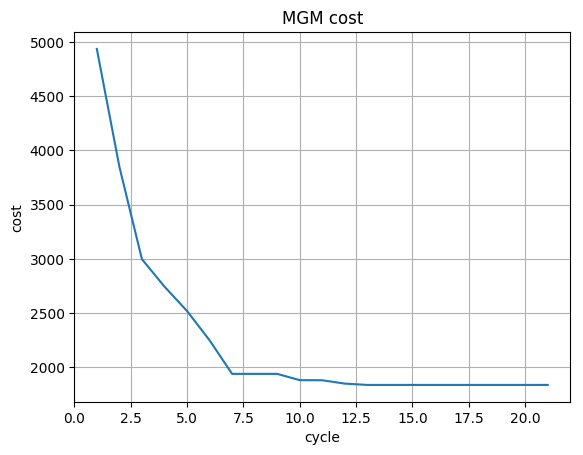
Fig. 1 MGM solution cost over 20 cycles.
Of course, before running this example, you need to install matplotlib:
pip install matplotlib
Logs
By default, the solve command (like all other
pyDCOP commands) only outputs the results (here, the end metrics) and does
not output any log, except if there are errors.
You can enable logs by adding the -v
global option with the requested level:
pydcop -v 2 solve --algo dpop graph_coloring.yaml
Level 1 displays only warnings messages, level 2 displays warnings and info messages and level 3 all messages (and can be quite verbose! )
For more control over logs, you can use the --log <conf_file>
option, where conf_file is a
standard python log configuration file:
pydcop --log algo_logs.conf solve --algo dpop graph_coloring.yaml
For example, using this long configuration file,
all log messages from DPOP computations will be output to an agents.log file,
without any log from the pyDCOP infrastructure
(discovery, messaging, etc.).
This can be very useful to analyse an algorithm’s behavior.
When solving our graph coloring problem with DPOP, you should get a log file
containing something similar to this:
pydcop.algo.dpop.v3 -  Leaf v3 prepares init message v3 -> v2
pydcop.algo.dpop.v2 -  Util message from v3 : NAryMatrixRelation(None, ['v2'], [-0.1  0.1])
pydcop.algo.dpop.v2 -  On UTIL message from v3, send UTILS msg to parent ['v3']
pydcop.algo.dpop.v1 -  Util message from v2 : NAryMatrixRelation(None, ['v1'], [0. 0.])
pydcop.algo.dpop.v1 -  ROOT: On UNTIL message from v2, send value msg to childrens ['v2']
pydcop.algo.dpop.v1 -  Selecting new value: R, -0.1 (previous: None, None)
pydcop.algo.dpop.v1 -  Value selected at v1 : R - -0.1
pydcop.algo.dpop.v2 -  v2: on value message from v1 : "DpopMessage(VALUE, ([Variable(v1, None, VariableDomain(colors))], ['R']))"
pydcop.algo.dpop.v2 -  Slicing relation on {'v1': 'R'}
pydcop.algo.dpop.v2 -  Relation after slicing NAryMatrixRelation (joined_utils, ['v2'])
pydcop.algo.dpop.v2 -  Selecting new value: G, 0.0 (previous: None, None)
pydcop.algo.dpop.v2 -  Value selected at v2 : G - 0.0
pydcop.algo.dpop.v3 -  v3: on value message from v2 : "DpopMessage(VALUE, ([Variable(v2, None, VariableDomain(colors))], ['G']))"
pydcop.algo.dpop.v3 -  Slicing relation on {'v2': 'G'}
pydcop.algo.dpop.v3 -  Relation after slicing NAryMatrixRelation(joined_utils, ['v3'])
pydcop.algo.dpop.v3 -  Selecting new value: R, 0.1 (previous: None, None)
pydcop.algo.dpop.v3 -  Value selected at v3 : R - 0.1